¶ Introduction to GrADS
GrADS (Grid Analysis and Display System) is a useful tool to read and write common data files (.csv, .nc) and create plots at the surface, lower and upper levels, and vertical profiles of datasets.
¶ Advantages
- open-sourced software
- user-friendly and recommended for beginners
- can open datasets commonly used in the lab
- several sample scripts and tutorials available online
¶ Disadvantages
- may be too rigid in handling special datasets such as model output
- few built-in functions
- not advisable for plots needing high statistics
¶ Tutorials
Note: This tutorial assumes the following:
- access to RCS computers
- basic programming (algorithms) for scripting
¶ Read and write files
¶ read a netCDF file
Run GrADS in your terminal:
$ gradsYou will get a prompt:
              Welcome to the OpenGrADS Bundle Distribution
              --------------------------------------------

For additional information enter "grads -h".

Starting "/opt/opengrads/Linux/Versions/2.1.0.oga.1/x86_64/grads   " ...


Grid Analysis and Display System (GrADS) Version 2.1.0.oga.1
Copyright (C) 1988-2016 by George Mason University
GrADS comes with ABSOLUTELY NO WARRANTY
See file COPYRIGHT for more information

Config: v2.1.0.oga.1 little-endian readline grib2 netcdf hdf4-sds hdf5 opendap-grids,stn athena geotiff shapefile cairo
Issue 'q config' command for more detailed configuration information
Loading User Defined Extensions table </opt/opengrads/Linux/Versions/2.1.0.oga.1/x86_64/gex/udxt> ... ok.
Landscape mode? ('n' for portrait): You may choose y for portrait or n for landscape mode.
This displays automatically in portrait (-p) or landscape (-l) format:
$ grads -p
$ grads -l A pop-up screen in black will appear based on the orientation chosen. Go back to the terminal, and the command line should have the symbol ga->.
GX Package Initialization: Size = 8.5 11
ga->To open a netCDF file, use the option sdfopen <filename>.nc:
ga-> sdfopen AphroTemp_V1204R1_1961_2007.nc
Scanning self-describing file:  AphroTemp_V1204R1_1961_2007.nc
SDF file AphroTemp_V1204R1_1961_2007.nc is open as file 1
LON set to 60.125 149.875
LAT set to -14.875 54.875
LEV set to 1 1
Time values set: 1961:1:1:0 1961:1:1:0
E set to 1 1
ga->This shows the APHRODITE temperature V1204R1latitude-longitude coordinates. The default setting of GrADS should open at the first time step (1961:1:1:0), and at the level nearest to surface (LEV set to 1 1).
To read the metadata of the APHRODITE netCDF, use q file:
ga-> q file
File 1 :
  Descriptor: AphroTemp_V1204R1_1961_2007.nc
  Binary: AphroTemp_V1204R1_1961_2007.nc
  Type = Gridded
  Xsize = 360  Ysize = 280  Zsize = 1  Tsize = 17166  Esize = 1
  Number of Variables = 2
     tave  1  t,z,y,x  daily mean temperature analysis interpolated onto 0.25deg grids [degC]
     rstn  1  t,z,y,x  ratio of 0.05deg-grids with station [%]
ga->The metadata shows that this file is Gridded, Zsize = 1 means that there is one level (at the surface), Tsize = 17166shows the time steps representing total days from 1961-2007. There are also two variables tave (daily mean temperature) and rstn.
To quickly display the variable tave in a map:
ga-> display tave
Contouring: -40 to 30 interval 5 and you should have a map over parts of Asia showing contour lines:
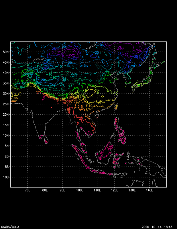
Note that this map represents the temperature at the first time step, specifically at January 1, 1961.
To close the file, type and enter quit:
ga-> quit
$ and you should be back to your terminal command line.
¶ read multiple netCDF files
Suppose you need to read two netCDF files. In this example, the reanalysis dataset ERA-Interim has two separate files for zonal winds (u10) and vertical winds (v10). Open GrADS:
$ grads -p

              Welcome to the OpenGrADS Bundle Distribution
              --------------------------------------------

For additional information enter "grads -h".

Starting "/opt/opengrads/Linux/Versions/2.1.0.oga.1/x86_64/grads   -p " ...


Grid Analysis and Display System (GrADS) Version 2.1.0.oga.1
Copyright (C) 1988-2016 by George Mason University
GrADS comes with ABSOLUTELY NO WARRANTY
See file COPYRIGHT for more information

Config: v2.1.0.oga.1 little-endian readline grib2 netcdf hdf4-sds hdf5 opendap-grids,stn athena geotiff shapefile cairo
Issue 'q config' command for more detailed configuration information
Loading User Defined Extensions table </opt/opengrads/Linux/Versions/2.1.0.oga.1/x86_64/gex/udxt> ... ok.
GX Package Initialization: Size = 8.5 11 Open the ERA-Interim zonal wind netCDF file (u10) which will be file 1:
ga-> sdfopen ein75_1986-2005_u10.nc
Scanning self-describing file:  ein75_1986-2005_u10.nc
SDF file ein75_1986-2005_u10.nc is open as file 1
LON set to 0 360
LAT set to -90 90
LEV set to 0 0
Time values set: 1986:1:1:0 1986:1:1:0
E set to 1 1
ga-> q file 1
File 1 :
  Descriptor: ein75_1986-2005_u10.nc
  Binary: ein75_1986-2005_u10.nc
  Type = Gridded
  Xsize = 480  Ysize = 241  Zsize = 1  Tsize = 240  Esize = 1
  Number of Variables = 1
u10 0 t,y,x 10 metre U wind componentThen, open ERA-Interim zonal wind netCDF file (v10). This will be file 2.
Note that you have to use q file 2 to display the metadata of file 2:
ga-> sdfopen ein75_1986-2005_v10.nc
Scanning self-describing file:  ein75_1986-2005_v10.nc
SDF file ein75_1986-2005_v10.nc is open as file 2
ga-> q file 2
File 2 :
  Descriptor: ein75_1986-2005_v10.nc
  Binary: ein75_1986-2005_v10.nc
  Type = Gridded
  Xsize = 480  Ysize = 241  Zsize = 1  Tsize = 240  Esize = 1
  Number of Variables = 1
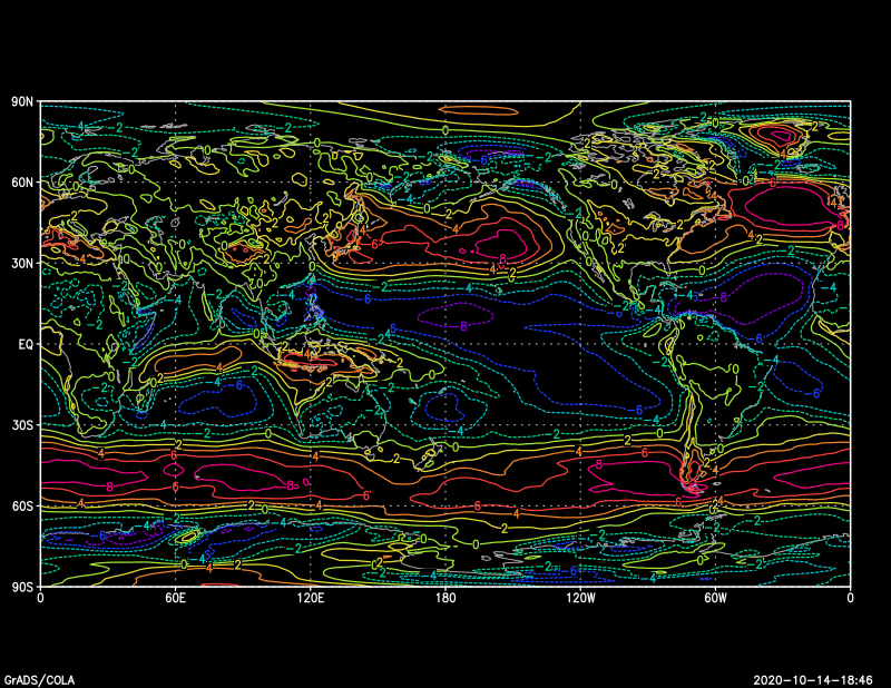
v10 0 t,y,x 10 metre V wind componentTo display the first time step of the file 1, use display <variable>.<file #>:
ga-> display u10.1Your pop-up screen should have a display like this:
So, to display the first time step of the file 2, the command should look like:
ga-> display u10.2Since we have a plot displayed previously, we need to clear first:
ga-> clearTo display wind vectors, there must be a u and v component. We need to skip some vectors so the figures are evenly spaced:
ga-> d skip(u10.1,10,10);skip(v10.2,10,10)Your plot should look like this:
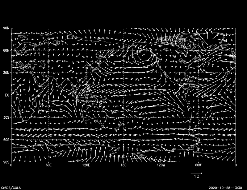
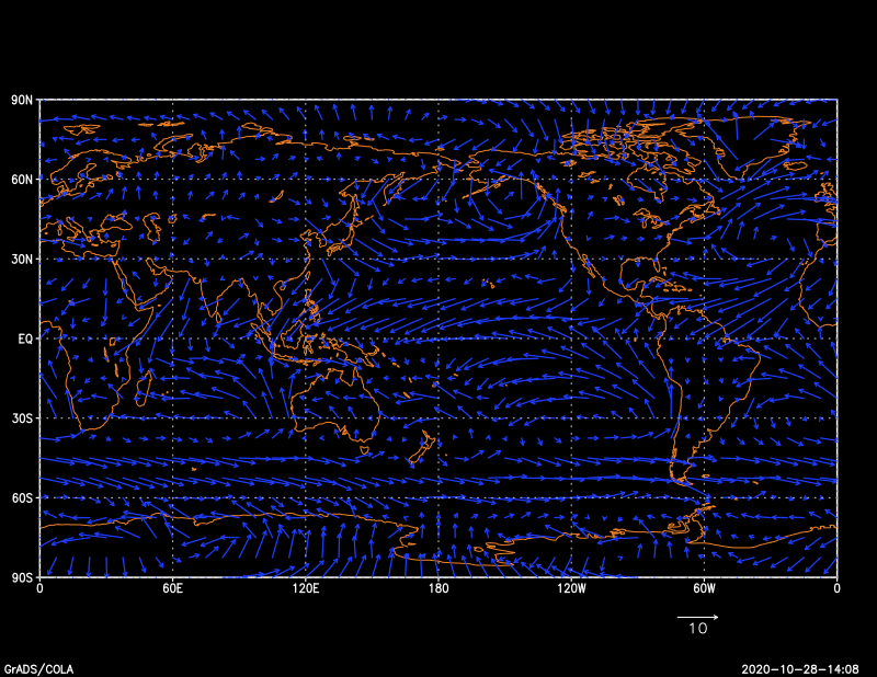
Since the wind vectors have the same color as the map, we can edit the vector color. In this example, we will set it to blue (set ccolor 4):
ga-> clear
ga-> set ccolor 4
ga-> d skip(u10.1,10,10);skip(v10.2,10,10)
¶ read .ctl files (coming soon!)
¶ write to .csv file
¶ write to .nc file
¶ Create plots: formatting and displaying a map
Note: these formats are usually done in scientific papers for your reference.
The plots in GrADs are made using a default size of a short bond paper (8.5" x 11") either in portrait or landscape orientation. The plots have a white background and they are properly labeled with a title and legend. Choice of colors is also important for communicating effectively.
For this example, we will plot seasonal mean daily precipitation over the Phlippines during Southwest Monsoon (June-September) using TRMM-3B42 dataset from 1998-2017. Note that the netCDF file is already prepared for the seasonal mean output via CDO (tutorial coming soon!).
In this sample GrADS is opened for landscape mode. Open the netCDF file and set coordinates for Philippine domain:
ga-> sdfopen 3B42_TRMM_Daily.1998-2017_JJAS.nc
ga-> set lat 5 21
ga-> set lon 115 130The following prepares the environment for a clean map with a white background and without the GrADs logo and grid guide lines (note: c = clear):
ga-> set display color white
ga-> c
ga-> set grads off
ga-> set grid offThis also ensures that the map plotted has coastal boarders in high resolution:
ga-> set mpdset hiresWe can plot the precipitation using the dataset resolution as pixelated (grfill) or smoothened (shaded). In this case, we choose the smoothened option.
ga-> set gxout shaded
ga-> d precipitationThe rainbow colors are default in GrADS. To complete the figure, we place the color bar and title:
ga-> cbar
ga-> draw title TRMM Daily Precipitation (JJAS 1998-2017) (mm/day)To finish, we print the image:
ga-> printim trmm_jjas_1998-2017.pngThe image is saved on your current working directory. The plot should look like this:
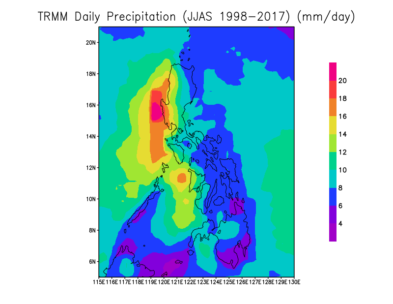
We expect that the highest rainfall amounts (> 20 mm/day) are located at the western part of the Philippines with climate type 1 based on the Coronas classification.
To improve the plot, we can change the size and interval of the lat/lon labels.
set xlopts <color> <thickness> <size>for setting x-axis label (in this case longitude) options where default is: color = 1, thickness = 3, size = 0.11set xlint <interval>for setting x-axis label interval (in this case how many degrees per interval)
For this example, we want to make the lat/lon coordinates labeled every 5 degrees with a larger font size:
ga-> c
ga-> set grads off
ga-> set xlopts 1 3 0.14
ga-> set xlopts 1 3 0.14
ga-> set xlint 5
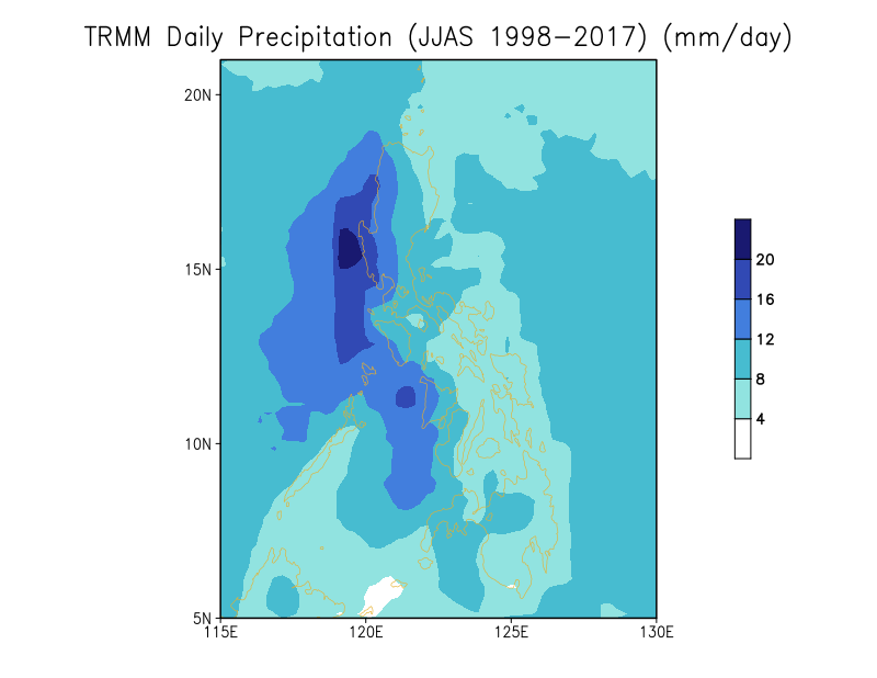
ga-> set ylint 5Regarding colors, precipitation is usually denoted in dark blue for wetter conditions, and light blue for less wet conditions. We first set the map coastline color to dark yellow (12) as contrast to the blue colors of precipitation:
ga-> set map 12Next, we can revise the plot with the function color.gs using user-defined colors and intervals.
color <min> <max> <interval> -kind color1->color2->color3->…->colorn
(Note: You may refer to Kodama's tutorial on the color names and other options for plotting.)
ga-> color 4 20 4 -kind white->mediumturquoise->royalblue->midnightblue
ga-> d precipitationTo improve the color bar, you may use Kodama's xcbar function with line on option to add outlines per color:
ga-> xcbar -line on
ga-> draw title TRMM Daily Precipitation (JJAS 1998-2017) (mm/day)
ga-> printim trmm_new.pngYour improved plot should look like this:
¶ masking land/ocean
In some datasets, values over land are missing (such as sea surface temperatures) or over ocean (such as in land cover categories), so a mask overlay is placed on the map for aesthetic purposes. Note, however, that the values below the mask overlay is not deleted.
The function used is basemap.gs:
basemap L(and)/O(cean) <fill_color> <outline_color> <L(owres)/M(res)/H(ires)>
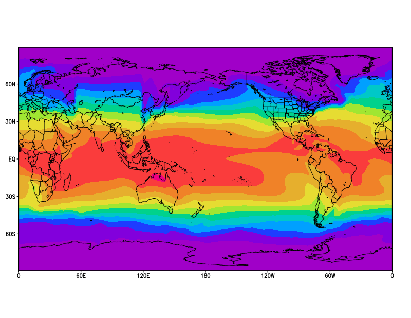
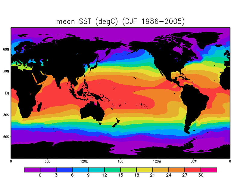
In this example, we will plot global mean sea surface temperatures (SST) from NOAA OISST dataset during boreal winter (DJF) from 1986-2005. In this case, the map dataset can be in medium resolution (mpdset mres):
ga-> sdfopen tos_oisst_1986-2005_DJF_1.nc
ga-> set display color white
ga-> c
ga-> set grads off
ga-> set grid off
ga-> set gxout shaded
ga-> set mpdset mresSince the dataset is in Kelvin, we convert the variable to Celsius:
ga-> d tos-273.15Your plot so far should look like this. Note that there are values over land that are unrealistic:
Recalling the syntax of basemap.gs, we will mask the values over land (L) in black color and outline (1) with medium resolution (M):
ga-> basemap L 1 1 M
ga-> xcbar -line on
ga-> draw title mean SST (degC) (DJF 1986-2005)
ga-> printim sst_final.pngYour plot should look like this:
¶ multiple plots in separate output files (requires scripts)
¶ multiple plots in one figure (panel) (requires scripts)
¶ Computing and statistics
¶ operators (+, -, *, /) (=, <, >, !=, <=, >=)
¶ commonly used functions
- mag(u,v)
- average (ave)
- area average (aave)
- regridding netCDF files (re)
¶ Student's T-test with hatches
¶ Sample Scripts
¶ how to run scripts
¶ read a file
¶ read multiple files
¶ write to .csv file
¶ write to .nc file
¶ formatting a map
¶ masking land/ocean
¶ multiple plots in separate output files
¶ multiple plots in one figure (panel)
¶ plotting wind speed
¶ area average (aave)
¶ regridding netCDF files (re)
¶ Student's T-test with hatches
¶ Useful Links
- http://cola.gmu.edu/grads/
- http://kodama.fubuki.info/wiki/wiki.cgi/GrADS/script?lang=en